Beyond the BI Graph Wizard

This post is aimed at BI Beans developers wanting to fully exploit all the features of the BI Beans Graph. Within JDeveloper the easiest way to create a new graph is to use the Graph Wizard. This will allow you to create a new query to populate the graph and also define the layout. The end result is an XML file within the BIDesigner. This XML file is stored on the local file system. Before deploying your application this XML file has to be copied to the remote catalog so your application can correctly locate and open it.

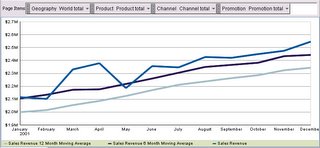
Once the graph has been created most of the properties relating to a graph are exposed using the customizer wizards that are part of the graph toolbar in JDeveloper. Using the GUI tools you can easily create a graph something like the one shown below, where the width of the lines has been increased and the colors for each line set to match a specific theme:

These are very basic customizations. However, the BI Beans graph does contain a lot of properties that are not covered by either the graph wizard or the customizers. There are three basic ways to access these additional properties:

1) Use the Structure and Properties panels in JDeveloper
2) Directly editing the graph XML file
3) Use the graph Java API

Method 1 : Using the Structure and Properties panels in JDeveloper

In JDeveloper the Structure and Properties panels can be used to view all the available graph properties. Once a graph is open in the JDeveloper graph editor, opening the Structure panel (Ctrl+Shift+S) will expose the all the structure of the graph bean:

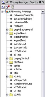
Some sections contain more detailed sections and are shown as drillable in the tree. For example the plotArea has an SFX section. This controls the Special Effects features. This is not exposed in the graph Wizard or the customizers, so the Properties panel has to be invoked to both view and modify these properties. To open the Properties panel use the (Ctrl+Shift+P) keystroke. The plotArea SFX has the following properties:

Using the SFX properties graph developers can add features such as background images to a graph. By setting the fillType, textureDisplay and textureURL properties it is easy to update the graph shown above by adding a background image as shown below:

In the actual graph XML file the following additional tags are added to control the SFX features:


Another feature that is only exposed via the Properties panel is the ability to wrap the text for the various title areas. In order to word-wrap long titles you simply select the required title in the structure panel, for example the Y1 Title:


The Property panel then exposes the options such as word wrap, text rotation, alignment etc. In the graph XML file the following entry would be added:

Method 2 : Directly editing the graph XML file

If you really want to push the boundaries the next step for customizing graphs is to directly edit the graph XML. As stated above, the graph definition is saved to an XML file within the BIDesigner directory on the local file store. Developers can use any text editor to open the file and add new XML tags or edit existing tags to customize the appearance of the graph. After saving the file, in JDeveloper you only need to reload the graph to view the results of the changes to the file.

The BI Beans graph is shipped with a DTD document that lists all the available XML tags. You can see the complete list of graph attributes inside the file 'graph.dtd'. This DTD file is located in your JDEVELOPER_HOME\bibeans\lib\bipres.jar. The WinZip utility can be used to unzip the contents of this JAR file and view the dtd document. For detailed information on these attributes, refer to the technical note available on OTN from the Reports Product Management Team:

http://www.oracle.com/technology/products/reports/htdocs/getstart/
whitepapers/graphdtd/graph_dtd_technote_2.html

This Technical Note explains all these attributes using comments within the graph.dtd. This document will help to explain the usage of these various attributes that provide more fine-grained customization of graphs.

Directly editing the XML provides more opportunities to customize the visual representations of a graph. For example, BI Beans Graph does not provide a graph type that just plots the trend as a series of floating bars. However, by directly editing the XML it is possible to generate a graph that does have floating bars as shown below:

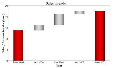
To do this is a two stage process. Assuming you have the following graph:

The first step is to add another series that clearly identifies the increase in sales for the years 2000-2002. Choose a stacked bar graph to show the two series. Your graph will now look like this:

Once this has been done, the next step is to add the following to the graph xml document:

The O1 axis tick mark style is defined so that the floating bars can be identified easily with their respective labels on the X-axis. The above XML entry will make one of the series transparent, and you will get a floating effect as shown below:

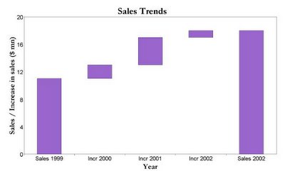
In order to show the total sales and increase in different colors, you will need to define exceptional risers. Exceptional risers are data markers that do not share series attributes, e.g., series color. Add the following to the Graph xml document to define exceptional risers:

This will change the color of the total sales bars as shown below:

To make the above graph look exactly like first graph with the nice red and silver bars some additional XML statements are required to modify the color codes used as part of the series definition and apply some special effects properties as well.

Method 3 : Using the graph Java API

The last method for interacting with the Graph bean is to use the Java API. This provides access to some interesting features such as the ability to set the bars or pie slices transparent. Currently the only way to set this property is to call the graph bean API using java code as follows:

DataAccess da = graph.getModel().getDataAccess();

int seriesCount = da.getEdgeExtent(DataDirector.ROW_EDGE);

for (int i=0; i

try{

graph.getSeries().setColor(new Color(red,green,blue,alpha), i);

}

catch (SeriesOutOfRangeException se){

System.out.println(" Series out of Bound Exception ");

}

}

This method uses the constructor for Color: Color(int r, int g, int b, int a) and creates an sRGB color with the specified red, green, blue, and alpha values in the range (0 - 255). The result is as follows:

Using BI Beans with non-OLAP data source

One of the largest threads currently running on the BI Beans forum relates to using BI Beans with non-OLAP data sources. Out of the box most of the BI presentation beans are wired to work with an OLAP data source. That OLAP data source can be derived from either a relational star/snowflake schema or an analytic workspace. The use of an OLAP data source against a relational schema requires additional metadata to be added in the form of registration of dimensions and cubes within the CWM repository.

In many cases the creation of this additional metadata may not be possible, so people have asked if it is possible to connect BI Beans to a non-OLAP data source. The answer is yes. The easiest way to do this is to use the BI Graph bean and connect this to an XML data source. This is relatively easy to do and as part of the BI Beans 10g samples we already provide a UIX example that shows how to connect a BI Graph bean to an XML data source. Now we have added a JSP example.

Using a very simple JSP page we can add a new BI Graph bean and render this with data from an XML data source. The code below shows the completed JSP page with all the require libraries and tags:

In this example the JSP page includes two key lines of code:

Line 1: helper.setGraphProperties(graph, "graph1.xml");
Line 2: helper.loadData(graph, false);

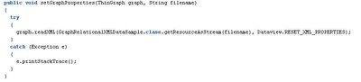
The first line sets the style properties for the graph. Below is the code used to load the style information and apply it to the graph:

For more information on setting the various graph properties and styles using the XML tags please refer to my previous posting “Beyond the BI Graph”. This can be found at the following URL:

http://all-siebel-info.blogspot.com/2008/05/beyond-bi-graph-wizard.html

The second line of code creates a connection to a non-OLAP data source for the graph and is contained within the same code library as the previous, code extract, GraphUIXSample.java. The loadData() method allows for two different types of connections. By passing the value of “false” as the last parameter the graph will be generated using data from an XML file, "helper.loadData(graph, false); ". This will call the following code:

This code loads an XML file that contains the following tags and data points:


which results in the following graph being displayed when the JSP is run:

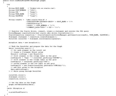
By passing the value of “true” as the last parameter ( helper.loadData(graph, true) )the graph will be generated using data from a SQL statement. This will call the following code:

For this example we connect to the Scott schema and select data from the EMP table. The connection details to the instance are coded into this example; however, these could be stored and loaded from another file if required. Note here the lack of a BIDesigner connection, this is an area that also generates a lot of questions on the forum. There is no need to define a BIDesigner to make a non-OLAP connection. The connection is defined as per a normal ODBC connection.

The SQL statement is contained within a String object and is defined as follows:

String sqlQuery = "select DEPTNO, JOB, avg(SAL)from EMP group by DEPTNO, JOB";

Executing the query in a SQLPlus session will generate the following result:

The query results are assigned to an array called “data” using a “while” loop to walk-through the result set. To assign the data to the graph the setTabularData() method is called:

graph.setTabularData(data);

Running the JSP page now will generate the same style of graph as before, however, the data will now be sourced from the EMP table and will appear as follows:

Multiple Conditional Formats on the same item

During a presentation today, I realized I didn't about this cool feature in Discoverer 10.1.2 till our UI and usability expert pointed it out.
When applying conditional formats in Discoverer (OLAP), you can have more than one conditional format active for a given item. As long as they do not overlap, they keep getting applied to the item, which means each successive format simply applies itself over and above the previous formats.

I always find it better to explain things using images and screenshots. So if you have understood what I am saying, the screenshots below are quite tautological.

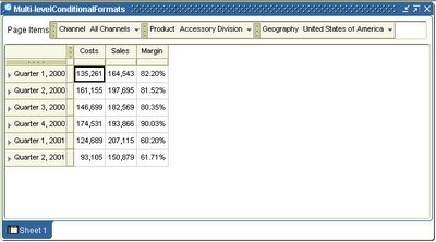
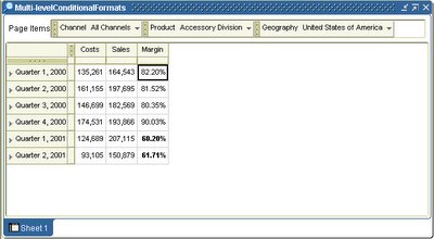
Take this worksheet I have created in Discoverer Plus OLAP. Quite straightforward; I have two measures - Costs and Sales, and one calculation - Margin.

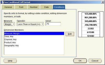
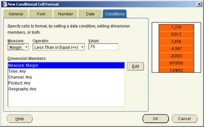
I now start applying a series of conditional formats to the 'Margin' calculation. Each format has the same condition, for simplicity: "Margin Less Than or Equal to 0.75" (i.e. 75%). For this first format, I simply state that the item should be formatted bold. The preview pane at the right shows me how this format would look like.
And this is how my worksheet looks like. Note that two cells in the 'Margin' column are now bold highlighted, corresponding to 'Quarter 1, 2001', and 'Quarter 2, 2001'.
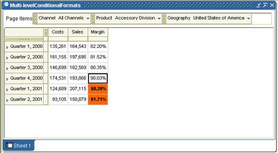
The second conditional format I apply is to format such cells (as meeting the "Margin Less Than or Equal to 0.75" condition) with a background of 'orange' (hex color code FF9900).
This background color format does not conflict with the earlier defined format, so all cells matching the condition get a background color of orange.

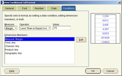
And finally I add a third conditional formt, with the same condition, but a different format. The font color is now set to be blue whenever the condition evaluates to true.
So now you can see below all three conditional formats existing in harmony, as none of the formats conflicts with the other.
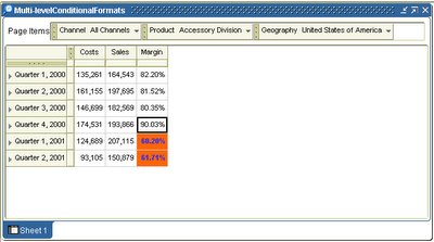
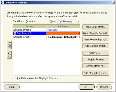
If you now take a look at all conditional formats (Format --> Conditional Formats), you shall see that all my three conditional formats are active.

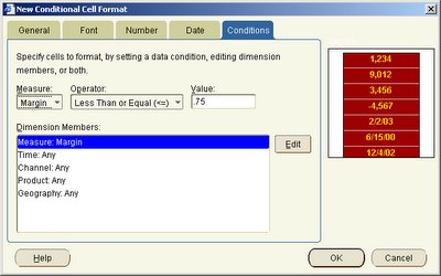
Let's now define a new conditional format, on the same item, that actually conflicts with an existing format. So, the fourth format I define still has the same condition (), but a format that conflicts with earlier formats: a cell background color of red and a foreground color of yellow (color:#FFCC00;background-color:#990000)
As I can see, this format now takes precendence over earlier defined conflicting formats.

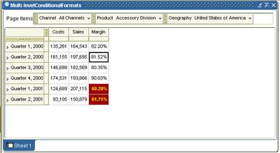
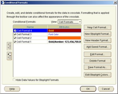
See the Conditional Formats list, and you will see that while all earlier formats for the item are still active, the last conditional format defined takes precedence, and hence conflicting formats are suppressed.

How Do You Debug OLAP DML from BI Beans?

Most BI applications simply provide read-only views on business data. However, some users do actually need to interact with data to perform data modeling and/or forecasting scenarios. Oracle’s OLAP environment provides an extremely rich and secure environment for providing this type of interaction. In a previous article in the Oracle magazine I explained how you to build a JSP page that allowed a user to select different types of forecasts. However, since SQL does not currently provide forecasting I used the multi-dimensional programming language OLAP DML, which is very similar to SQL.

In the process of creating this sample I discovered a number of issues that lead to some new features within BI Beans 10g. Most of the issues of combining server side programming (OLAP DML) with JSP development is actually debugging the whole stack. JDeveloper provides excellent JSP debugging tools and the JDev team have some excellent samples that can be found on their OTN home page.

However, trying to debug OLAP DML was not quite as easy. So as part of BI Beans10g we provided some additional debugging facilities to help OLAP DML developers. A generic AW is used to debug any OLAP DML operation that is called from a JSP page. This AW is shipped as part of the Common Schema samples and is usually installed into the CS_OLAP schema and is called AWDEBUG. It contains a program that controls the whole debug process, called BI_BEANS_UTIL. That program takes the following arguments:

• Context Name passed from Java Environment
• Current directory setting
• Name of calling program
• Mode of operation - START or STOP
• Should prgtrace be enabled
• Should badline be enabled
• Should monitor be enabled
• Should trackprg be enabled

The AWProgram JSP tag controls many of these arguments. The JSP tag has properties that allow the developer to control which of the features are enabled or disabled.

To show how the debugging process works lets review the What-If JSP page that is part of the Executive Insight demo. The page contains two buttons above the bar graph:

• Run Model – executes a new forecast using the OLAP DML program RUN_MODEL
• Reset – clears forecasted data using the OLAP DML program CLEAR_DATA

To enable the debugging process the AWDEBUG workspace needs to be attached to the current session. This is done using an AWCommand tag. The tag is added to the start of JSP page and is set to manually execute. Other options are “onRender” or “onInit” and these are self-explanatory.

The wizard that defines the tag allows the developer to type any OLAP DML command into a window. These are the commands that will be executed when the tag is called.

For this example, we attach the AW UTILS that contains the programs that will create the forecast data and also remove the forecast data for the “Reset” button. The second command attaches the AW that controls debugging.

The next step is to add the two buttons that will execute the OLAP DML and update the graph with the new data. These buttons can be defined using the AWProgram JSP Tag. The tag wizard prompts for the required inputs. The key fields are as follows:

• debugPath – this is the name of a directory object created within the database instance and points to a directory path on the server. All trace files will be written to this directory
• ShowTrace – enable trace of each line of code. This sets the OLAP DML option called PRGTRACE. This generates a file called program_name_PRGTRACE_timestamp.trc
• ShowBadLine – enables verbose error messages
• ShowMonitor – enables recording of execution timings of each line of code. This generates a file called program_name_MONITOR_timestamp.trc
• ShowTrackprg - enables recording of execution timings of each program. This generates a file called program_name_TRACK_timestamp.trc

Each file is written to the directory specified in the debugPath property. All tracing is enabled only for the duration of the execution of the tag. Once the tag has finished firing all tracing is automatically disabled.

The three files that are generated contain different information and are used to debug different situations. Once an OLAP DML program has been defined the next step is to ensure it is executing correctly. The execution path can be traced using the showTrace property. This will show, line by line, the flow of the program. Assuming the program is running correctly but performance is not as expected you can use the showTrackprg and showMonitor properties to evaluate how much time is being spent within each program and on each line within each program. This can highlight lines of code that are taking a long time to execute and that need optimizing. I will provide a detailed review of each of these trace files in the next article.